RNN for sequence-to-sequence classification

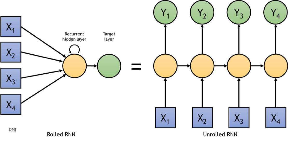
In order to understand a sequence of information we need to understand each input of data based on the understanding of previous data. We can’t throw everything away and start processing another sequence. This is the major idea behind RNNs.

Traditional neural networks cannot do this, which appears to be a significant limitation. Assume you want to categorise what type of event is occurring at each point in a movie. It’s unclear how a traditional neural network could use previous events in the film to inform subsequent ones.

Recurrent neural networks address this issue. They are networks with loops in them, allowing information to persist. RNNs were first introduced in the paper, “Learning internal representations by error propagation” (1984) and they revolutionalized the way we do speech recognition, language modelling, translation, image captioning etc. In this article we will be going over how to model simple RNNs, GRUs, LSTM and Bidirectional LSTM to predict heart disease (binary classification) for sequential data.

Data Preparation and Import

Our dataset is already standardised as seen in Figure 1. It has a total of 140 columns and 1621 rows.

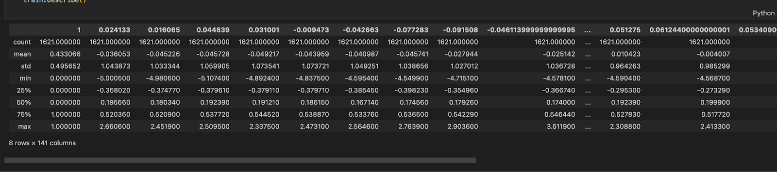
The code block below shows how we have stored our data in a dataframe inside of separate dictionaries.

transformed_df = {"X_train": [], "Y_train": [], "X_test": [], "Y_test": []}
transformed_df["X_train"] = dataset_train.drop("1", axis=1)
transformed_df["Y_train"] = dataset_train["1"]

transformed_df["X_test"] = dataset_test.drop("1", axis=1)
transformed_df["Y_test"] = dataset_test["1"]

While we have not done any normalization or standardization to our data (because the data is already standardized), it’s important to do so for a Recurrent Neural Network. Why is normalising or standardizing our data necessary? It’s because the order of magnitude of the characteristics can affect the performance of some models. Some models might “believe” that one characteristic is more significant than another if, for instance, one feature has an order of magnitude equal to 1000 and another has an order of magnitude equal to 10. The order of magnitude doesn’t tell us anything about the predictive power, hence it is biased. We may eliminate this bias by changing the variables to give them the same order of magnitude.

Standardization and normalisation are two of these transformations, which convert each variable into a 0–1 interval (which transforms each variable into a 0-mean and unit variance variable). Standardisation, theoretically, is superior to normalisation because it does not cause the probability distribution of a variable to shrink in the presence of outliers

Building the model: Simple RNN

RNNs were first introduced in the paper, “Learning internal representations by error propagation” (1984). The first layer in this model will be a simple RNN layer. Then there is a Dropout layer followed by 2 more sets of the same architecture. We have a Flatten and Dense layer near the end. The model is shown below.

model = keras.Sequential([
 keras.layers.SimpleRNN(units=50, return_sequences= True),
 keras.layers.Dropout(0.2),
 keras.layers.SimpleRNN(units=50, return_sequences= True),
 keras.layers.Dropout(0.2),
 keras.layers.SimpleRNN(units=50, return_sequences= True),
 keras.layers.Dropout(0.2),
 keras.layers.Flatten(),
 keras.layers.Dense(10, activation='relu'),
 keras.layers.Dense(1, activation='sigmoid')
])

model.compile(loss='binary_crossentropy',
 optimizer='adam',
 metrics=['accuracy'])
model.build(X_train.shape)

callback = keras.callbacks.EarlyStopping(monitor="val_loss",
 min_delta=0,
 patience=3,
 verbose=1,
 mode="auto",
 baseline=None,
 restore_best_weights=True)
history_gru = model.fit(x=X_train,y=Y_train, validation_split=0.20, batch_size=32, epochs=30, verbose=2, callbacks=[callback])

The input shape of the SimpleRNN layer in the first layer is 32, and the output shape is also 32. We have compiled the model using the binary crossentropy loss function, the ‘adam’ optimizer, and the accuracy metric. We have also used Early Stopping to minimize validation loss. Early stopping is an innovative method for regularising a machine learning model. It achieves this by stopping training when the validation error is at a minimum.

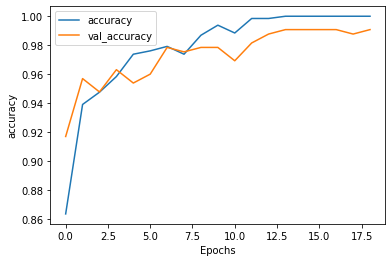
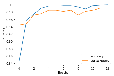
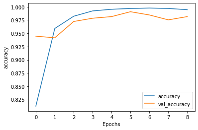
After 12 epochs training accuracy becomes 98.84 while validation accuracy reaches 98.85. This is shown in Figure 2.2.

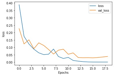
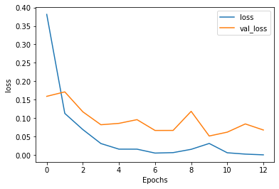
The training loss in the meantime decreases to 0.3034 and the validation loss reduces to 0.2796. This is shown in Figure 3.

Model Evaluation

**Figure 4 **shows how well our last model, i.e, Simple RNN performed and how well it approximates the relationship between having a disease and not having a disease through the use of the Confusion Matrix.

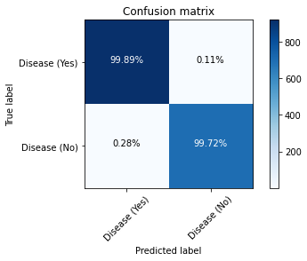
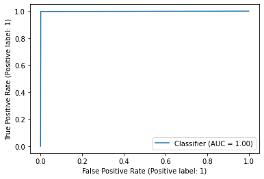
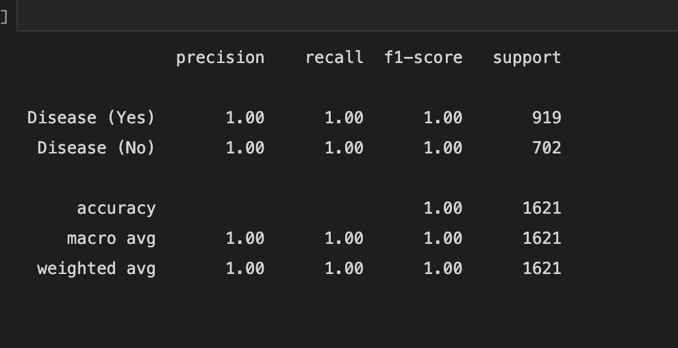
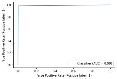
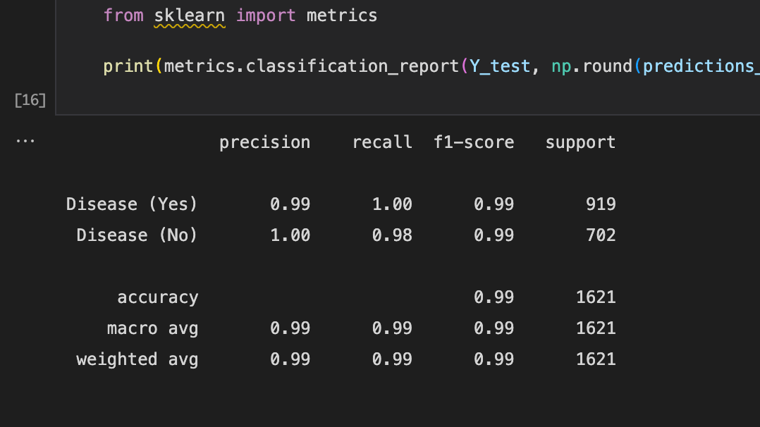
**Figure 5 **shows the ROC curve and **Figure 2.6 **reports the model’s performance against a range of metrics such as Precision, recall, Accuracy and F1-score.

Building the model: GRU

The second model that we have developed is a Gated Recurrent Unit which is a variation of the LSTM. Introduced by Cho, et al. (2014). It combines the forget and input gates into a single “update gate.” The first layer in this model will be a Bidirectional GRU layer. Then there is a Dropout layer followed by 2 more sets of the same architecture. We have a Flatten and Dense layer near the end. The model is shown below.

model = keras.Sequential([
 keras.layers.Bidirectional(keras.layers.GRU(units=50, return_sequences= True)),
 keras.layers.Dropout(0.2),
 keras.layers.Bidirectional(keras.layers.GRU(units=50, return_sequences= True)),
 keras.layers.Dropout(0.2),
 keras.layers.Bidirectional(keras.layers.GRU(units=50, return_sequences= True)),
 keras.layers.Dropout(0.2),
 keras.layers.Flatten(),
 keras.layers.Dense(10, activation='relu'),
 keras.layers.Dense(1, activation='sigmoid')
])

model.compile(loss='binary_crossentropy',
 optimizer='adam',
 metrics=['accuracy'])

model.build(X_train.shape)

callback = keras.callbacks.EarlyStopping(monitor="val_loss",
 min_delta=0,
 patience=3,
 verbose=1,
 mode="auto",
 baseline=None,
 restore_best_weights=True)

history_rnn = model.fit(x=X_train,y=Y_train, validation_split=0.20, batch_size=32, epochs=30, verbose=2, callbacks=[callback])

The input shape of the GRU layer in the first layer is 32, and the output shape is also 32. We have compiled the model using the binary crossentropy loss function, the ‘adam’ optimizer, and the accuracy metric. Early Stopping has been used in this model as well.

After 13 epochs training accuracy becomes 98.84% while validation accuracy reaches 98.15%. This is shown in Figure 7.

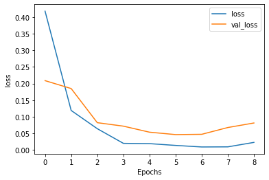
The training loss in the meantime decreases to 0.03 and the validation loss reduces to 0.05. This is shown in Figure 8.

Model Evaluation

**Figure 9 **shows how well our last model, i.e, GRU performed and how well it approximates the relationship between having a disease and not having a disease through the use of the Confusion Matrix.

**Figure 10 **shows the ROC curve and **Figure 11 **reports the model’s performance against a range of metrics such as Precision, recall, Accuracy and F1-score.

Building the model: Bidirectional LSTM

The third and final model that we have developed is a Bidirectional LSTM which is again a variation of the LSTM. Long Short Term Memory networks, also known as “LSTMs,” are a type of RNN that can learn long-term dependencies. Hochreiter and Schmidhuber (1997) introduced them, and many people refined and popularised them in subsequent work. They work extremely well on a wide range of problems and are now widely used.

The first layer in this model will be a Bidirectional LSTM layer. Then there is a Dropout layer followed by 2 more sets of the same architecture. We have a Flatten and Dense layer near the end. The model is shown below.

model = keras.Sequential([
 keras.layers.Bidirectional(keras.layers.LSTM(units=50, return_sequences= True)),
 keras.layers.Dropout(0.2),
 keras.layers.Bidirectional(keras.layers.LSTM(units=50, return_sequences= True)),
 keras.layers.Dropout(0.2),
 keras.layers.Bidirectional(keras.layers.LSTM(units=50, return_sequences= True)),
 keras.layers.Dropout(0.2),
 keras.layers.Flatten(),
 keras.layers.Dense(10, activation='relu'),
 keras.layers.Dense(1, activation='sigmoid')
])

model.compile(loss='binary_crossentropy',
 optimizer='adam',
 metrics=['accuracy'])

model.build(X_train.shape)

The input shape of the LSTM layer in the first layer is 32, and the output shape is also 32. We have compiled the model using the binary crossentropy loss function, the ‘adam’ optimizer, and the accuracy metric. Early Stopping has been used in this model as well.

After 13 epochs training accuracy becomes 99.69% while validation accuracy reaches 99.08%. This is shown in Figure 12.

The training loss in the meantime decreases to 0.03 and the validation loss reduces to 0.05. This is shown in Figure 13.

Model Evaluation

**Figure 14 **shows how well our last model, i.e, LSTM performed and how well it approximates the relationship between having a disease and not having a disease through the use of the Confusion Matrix.

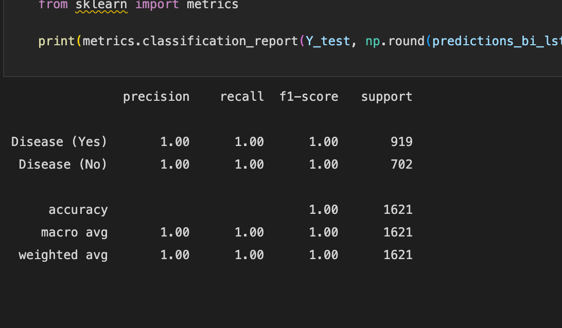
**Figure 15 **shows the ROC curve and **Figure 16 **reports the model’s performance against a range of metrics such as Precision, recall, Accuracy and F1-score.

Justification and Model Evaluation

Short-term Memory Is a Problem

Short-term memory is a problem for recurrent neural networks. They will have difficulty carrying information from earlier time steps to later ones if the sequence is long enough. So, if you’re trying to predict something from a paragraph of text, RNNs may leave out important information at the start.

The vanishing gradient problem affects recurrent neural networks during backpropagation. Gradients are values that are used to update the weights of a neural network. The vanishing gradient problem occurs when the gradient shrinks as it propagates backwards in time. When a gradient value becomes extremely small, it does not contribute significantly to learning.

LSTMs and GRUs as a solution

As a solution to short-term memory, LSTMs and GRUs were developed. They have internal mechanisms known as gates that allow them to control the flow of information. These gates can learn which data in a sequence should be kept or discarded. This allows it to pass relevant information down the long chain of sequences in order to make predictions. Almost all state-of-the-art recurrent neural network results are achieved with these two networks. To summarise, RNNs are good for processing sequence data for predictions but have a short-term memory problem. LSTMs and GRUs were developed to mitigate short-term memory using mechanisms known as gates. Gates are simply neural networks that control the flow of information through the sequence chain.

Evaluation: RNN vs GRU vs LSTM

As we can see from the experimentation results, all the models give out nearly 100% accuracy when trained with a similar network architecture. The one big difference that we have noticed is the training time required to train Simple RNN is a lot more compared to the GRU and the LSTM model.

Based on how all the models, RNN, LSTM and GRU, work, GRU uses fewer training parameters and thus uses less memory and executes faster than LSTM, whereas LSTM is more accurate. RNN on the other hand uses the most memory and executes the slowest. We can conclude that when dealing with large sequences and accuracy is important, LSTM should be used; GRU should be used when less memory is available and faster results are desired.

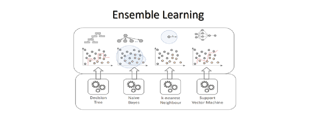
RNNs vs Ensemble Learning

As we have seen in our experimental results shown in Figure 1 and **Figure 4 of this article , **the accuracy of our Ensemble classifier barely beats out the accuracy of our RNN model. At the same time, the amount of time and CPU resources required to train the RNN model are substantially more than the Voting Classifier created for the Ensemble learning task. For comparison, RNN took an average of 400ms for every epoch with a total of 19 epochs. Our Voting Classifier on the other hand barely took a second to train and fit the data.

Some key takeaways from constructing and analysing both models are

Easier to interpret: Because classical ML employs direct feature engineering, all the algorithms used in the Voting Classifier are simple to interpret and comprehend. Furthermore, because we have a better understanding of the data and underlying algorithms, tuning hyper-parameters and changing model designs is easier. RNN, on the other hand, is a “black box” in the sense that we do not fully understand the “inside” of deep networks even now. Because of the lack of theoretical foundation, hyper-parameters and network design are also quite difficult.

Training time and computational costs: RNNs require high-end GPUs to be trained in a reasonable amount of time with big data, both financially and computationally. These GPUs are very expensive, but training deep networks to high performance would be impossible without them. A fast CPU, SSD storage, and fast and large RAM are all required to effectively use such high-end GPUs. Classical ML algorithms, such as BN, KNN, EL and SVM can be trained with a decent CPU without the need for cutting-edge hardware. Because they are less computationally expensive, they allow us to iterate faster and try out more techniques in less time.

Ensemble Learning perform better on small datasets: Deep networks require extremely large datasets to achieve high performance. Such large datasets are not readily available for many applications and will be costly and time-consuming to acquire. While our provided dataset is very small, we can still see that Classical ML algorithms, i.e, BN, KNN, EL and SVM outperform RNN on a smaller dataset.

Adaptability: RNNs are far more adaptable and transferable than Ensemble Learning algorithms in terms of domains and applications. The RNN we have built can easily be transferable for a multitude of different tasks, such as speech recognition, language modelling, translation, image captioning etc. Ensemble Learning and other classical machine learning algorithms are not as flexible and require extensive study and knowledge before applying it to a new field. The classical ML knowledge base for different domains and applications is quite different and frequently necessitates extensive specialised study within each individual area.

Conclusion

RNN, GRU and LST were used in the development of our Binary Classification models. When trained on a similar architecture, all of the models gave similarly high accuracy of about ~99%. Though RNNs proved to be slower compared to the newer LSTMs and GRUs, the accuracy of our Binary classifier was not affected.

References

1. GitHub: https://github.com/nandangrover/recurrent-neural-network

2. Schuster, M., & Paliwal, K. K. (1997). Bidirectional recurrent neural networks. IEEE Transactions on Signal Processing, 45(11), 2673–2681. https://doi.org/10.1109/78.650093

3. Dey, R., & Salem, F. M. (n.d.). Gate-Variants of Gated Recurrent Unit (GRU) Neural Networks.

4. Ruineihart, D. E., Hint, G. E., & Williams, R. J. (1985). LEARNING INTERNAL REPRESENTATIONS BERROR PROPAGATION two.