Heart Disease Detection using fastai and sklearn

Since I began my master’s programme in artificial intelligence, I’ve been looking for a framework that will help me use my software development skills a lot more, design systems that are ready for production, and wrap some of the repetitive, everyday ML code around a framework that just works. Fastai, a tool that builds multilayer neural networks in only a few lines of code and has Pytorch as its backbone, has the power to do just that.

In 2015 the idea of creating a computer system that could recognise birds was considered so outrageously challenging that it was the basis of this XKCD joke .

Using fastai it’s a matter of writing a couple of lines of code to build a Convolutional Neural Network that can recognize birds with more than ~95% accuracy.

In this article we will explore how we can build a Heart Disease Detection system using Decision Trees, Random Forest, Gradient Bossting and a Neural Network. We will do all of this while using fastai for some of the mundane tasks such as data cleaning, feature engineering, data visualization and model evaluation. The jupyter notebook and the data set can be found in this repository: nandangrover/heart-disease-classifier .

Describing the dataset

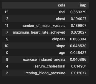
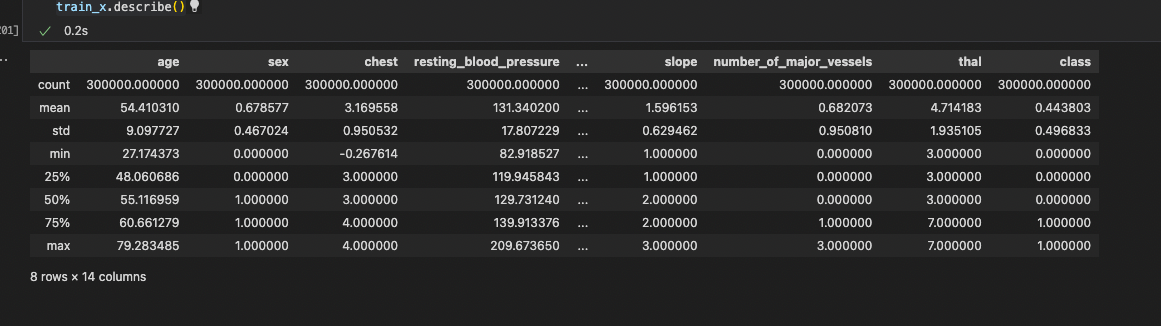
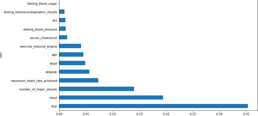
Figure 2.2.2 gives a brief overview of the dataset provided. The total number of features present is 13 (we have added a class in the same dataframe for our preprocessing). The number of examples present is 30,000 in the train and 30,000 in the test dataset. After exploring the dataset, we could see that the data is clean with no missing values. Feature engineering was applied to the dataset as shown in Figure 2.2.4. Exploratory data analysis showed us that thal has the most impact on the predictions while resting_blood_pressure has the least impact on heart disease prediction. The total impact of every feature is listed out below in Figure 2.2.1.

Building the model

Decision tree ensembles, as the name suggests, rely on decision trees. A decision tree asks a series of binary (that is, yes or no) questions about the data. After each question, the data at that part of the tree is split between a “yes” and a “no” branch, as shown in Figure 2.2.3. After one or more questions, either a prediction can be made on the basis of all previous answers or another question is required. In terms of processing time and scalability, they do classification much better than neural networks as we will see down below.

test_x = pd.read_csv('data/x_test.csv', low_memory=False)
test_y = pd.read_csv('data/y_test.csv', low_memory=False)

We start by importing the data using panda as shown above**.**

In order to visualize our Decision Tree model we first build a model with max_lead_nodes set to 10.

model = DecisionTreeClassifier(max_leaf_nodes=10)
model.fit(xs, y);

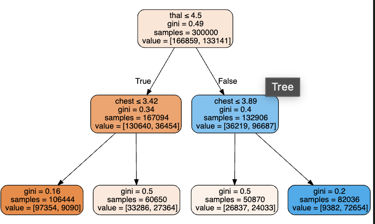
The top node represents the initial model before any splits have been done, when all the data is in one group. This is the simplest possible model. It is the result of asking zero questions and will always predict the value to be the average value of the whole dataset.

model_decision = DecisionTreeClassifier(min_samples_leaf=25)
model_decision.fit(xs, y)
cross_val_score(model_decision, valid_xs, valid_y, cv=10)

Sklearn’s default settings allow it to continue splitting nodes until there is only one item in each leaf node. Therefore, we change the min_sample_leaf setting to 25, so that our model doesn’t overfit. The accuracy without the min_sample_leaf specified was also measured, which came at a lowly 86%.

array([0.86806667, 0.86516667, 0.8636    , 0.8647    , 0.86746667, 0.8649    , 0.86413333, 0.86556667, 0.86706667, 0.86486667])

After setting the min_sample_leaf to 25, the cross-validation accuracy for 10 epochs is given below.

array([0.88946667, 0.88743333, 0.8857    , 0.89053333, 0.88933333, 0.8873    , 0.8874    , 0.88836667, 0.88936667, 0.88643333])

We see an average accuracy of around 89% for the decision tree. In the next section, we will see if removing the low-importance variables has any effect on the accuracy

Accuracy of the Decision Tree with Low-Importance Variables Removed

We want to know how a model is producing predictions in addition to merely knowing that it can do it accurately. This is revealed by feature significance. By looking at the feature importances_ attribute, we can obtain these directly.

def rf_feat_importance(model, df):
   return pd.DataFrame({'cols':df.columns, 'imp':model.feature_importances_}
                      ).sort_values('imp', ascending=False)

By eliminating the factors of low value, it appears plausible that we might employ just a portion of the columns and still achieve good results. So we have gone ahead and removed all the features with importance less than 0.005 (Figure 2.2.4).

We observe that the accuracy remains the same after removing the features which are of low importance.

array([0.88943333, 0.88733333, 0.88553333, 0.89046667, 0.88896667, 0.8874    , 0.88736667, 0.88873333, 0.88933333, 0.88643333])

Model Evaluation

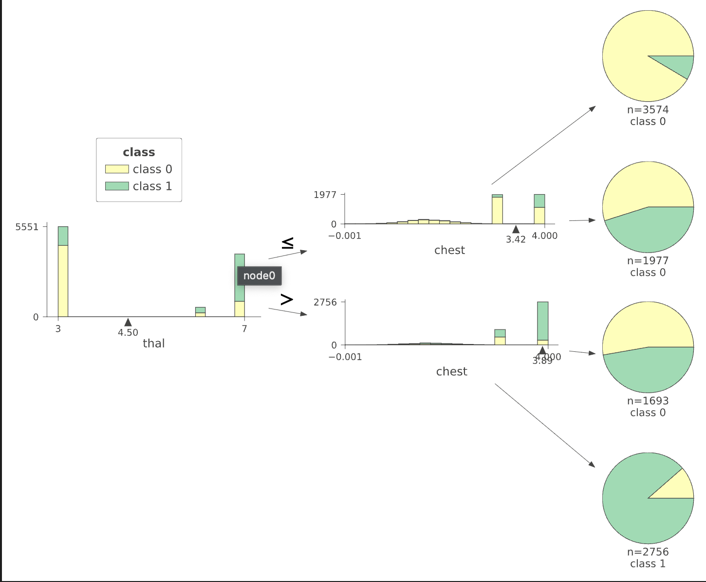
We can visualize how the data is split from the first column thal and then chest for the first four leafs. We can see that the decision tree algorithm has successfully split using thal value into two more groups which differ in value significantly. This is possible using Terence Parr’s powerful dtreeviz library (Figure 2.2.5).

Random Forest, Gradient Boosting and Neural Network

We have built a classifier using an ensemble of decision trees, i.e, using Random Forest algorithm and Gradient Boosting. A neural network was also built in order to compare the accuracy, scalability, time taken and effort required to implement Decision trees.

Random Forest

The following function specification specifies the number of estimators we want, the maximum number of rows to sample for each tree’s training, and the maximum number of columns to sample at each split point (where 0.5 means “take half the total number of columns”). The same min samples leaf parameter we used for decision trees can also be used to define when to stop splitting the tree nodes, so limiting the depth of the tree. Finally, we instruct Sklearn to create the trees concurrently by passing n jobs=-1. The final accuracy achieved as a result was 90%.

def rf(xs, y, n_estimators=200, max_samples=200_000,
      max_features=0.5, min_samples_leaf=10, **kwargs):
   return RandomForestClassifier(n_jobs=-1, n_estimators=n_estimators,
       max_samples=max_samples, max_features=max_features,
       min_samples_leaf=min_samples_leaf, oob_score=True).fit(xs, y)

Gradient Boosting

We have used HistGradientBoostingClassifier which has native support for missing values (NaNs). During training, the tree grower learns at each split point whether samples with missing values should go to the left or right child, based on the potential gain. When predicting, samples with missing values are assigned to the left or right child consequently. If no missing values were encountered for a given feature during training, then samples with missing values are mapped to whichever child has the most samples. The final accuracy achieved as a result was 90%

model_gradient = HistGradientBoostingClassifier().fit(xs_imp, y)

Neural Network

With over 60,000 examples and 5 epochs the network was introduced to over 300,000 examples. This is a lot of data for a neural network to learn from. The accuracy of the neural network is 0.55 which is lower than the decision tree because of the limited hardware resources (by limited I mean 80GB of ram and a TPU from Google collab). The neural network is also slower than the decision tree. We have used fast AI’s tabular_learner to build the neural network. By default, it uses 2 layers with a first layer having 200 activations and the second layer having 100 activations. We decided to go with the defaults since we are comparing Neural Nets with decision trees and not actively trying to increase the accuracy. The final accuracy achieved as a result was 55.75%, which can be improved by tweaking the learning rate (using lr_find() method of fastai) and train the model for more epochs.

df = TabularPandas(combined_data, procs_nn, list(to_keep), [], y_names='class', splits=splits)
dataLaoders = df.dataloaders(64)

learn = tabular_learner(dataLaoders)

if os.path.exists('data/models/nn'):
 learn.load('data/models/nn.pkl')
else:
 learn.fit_one_cycle(5, 1e-2)

References

• Codebase: nandangrover/heart-disease-detection

• Fast AI course: https://course.fast.ai

• Quinlan, J. R. (1986). Induction of Decision Trees. In Machine Learning (Vol. 1).

• Zhang, N. L., Qi, R., & Poole, D. (1993). A Computational Theory of Decision Networks. In International Journal of Approximate Reasoning (Vol. 11).